rfa module

Recreate from average function with given strategy.

class AbstractRFA(x, y, n, **kwargs)

Bases: ABC

Abstract class for recreating from average (RFA) a function y measured in x.

To perform recreate from average, call rfa() method, which returns newly created points.

By default, x axis is oversampled with n linearly space values between each point. To change this behaviour, override _initial_x_oversample method.

By default, y axis is oversampled with n piecewise constant values between each point. To change this behaviour, override _initial_y_oversample method.

The rfa() method returns recreated function values for x and y.

In the following derived classes, term ‘interval’ refers to the distance between two consecutive observations (values in y based on x). Each interval contains n samples obtained by oversampling.

Parameters:

x (1-D array-like) – Independent variable in strictly increasing order.
y (1-D array-like) – Dependent variable.
n (int) – Number of points oversampled and recreated in the function for each interval. Cannot be lower than 2.
**kwargs (dict) – Arbitrary keyword arguments for concrete implementations.

See also

IntervalArray()

abstract rfa()

Recreate function from average on x and y variables.

Returns:

xs (ndarray) – Oversampled independent variable x.
ys (ndarray) – Oversampled dependent variable y.

class PiecewiseConstantRFA(x, y, n, **kwargs)

Bases: AbstractRFA

Recreate function using piecewise constant values.

rfa()

Recreate function from average on x and y variables.

Returns:

xs (ndarray) – Oversampled independent variable x.
ys (ndarray) – Oversampled dependent variable y.

class FunctionRFA(x, y, n, sampling_function_supplier=None, sampling_function_supplier_kwargs=None)

Bases: AbstractRFA

Recreate function using created sampling function.

Created sampling function should take x as an argument and return corresponding y value.

Sampling function can be specified by overriding _get_sampling_function() method. If method is not override sampling_function_supplier factory is used to produce a sampling function.

Parameters:

x (1-D array-like) – Independent variable in strictly increasing order.
y (1-D array-like) – Dependent variable.
n (int) – Number of points oversampled and recreated in the function.
sampling_function_supplier (Callable[[np.ndarray, np.ndarray], Callable]) – Factory that takes an input x and y points and creates a new function f(float) -> float. New function takes any arbitrary point as an input, and returning its corresponding value as an output.
sampling_function_supplier_kwargs (dict, optional) – Kwargs passed to sampling_function_supplier.

rfa()

Recreate function from average on x and y variables.

Returns:

xs (ndarray) – Oversampled independent variable x.
ys (ndarray) – Oversampled dependent variable y.

class CubicSplineRFA(x, y, n, sampling_function_supplier=<function CubicSplineRFA.<lambda>>)

Bases: FunctionRFA

Recreate function using cubic spline between given points.

class IntervalRFA(x, y, n, **kwargs)

Bases: AbstractRFA

Abstraction for interval based function recreate from average classes.

class LinearFixedRFA(x, y, n, alpha=1.0, a=None)

Bases: AbstractRFA

Linearly moves between points in fixed transition intervals.

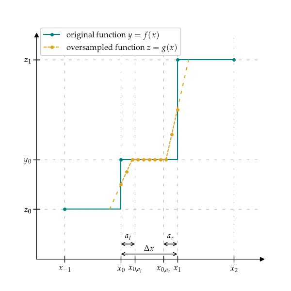
Transition linearly between intervals in transition window (part of the interval). Transition window is defined in number of samples a and divided proportionally to the left and right side of the interval. If a is not specified, it is obtained based on the transition samples factor alpha multiplied by the number of inserted samples for each interval n. a cannot be lower, than 2 samples. If it is, it’s value is changed to correct that.

Parameters:

x (1-D array-like) – Independent variable in strictly increasing order.
y (1-D array-like) – Dependent variable.
n (int) – Number of points oversampled and recreated in the function.
alpha (float, default: 1.0) – Transition window samples factor for moving between intervals.
a (int, optional) – Transition window samples for moving between intervals. If not specified, it is equal to alpha * n. Cannot be lower than 2.

Notes

Let us consider k-th interval and \(x_{k,i}\), \(y{k,i}\) refer to i-th sample of k-th interval for x and y, respectively. When omitting value, e.g., \(x_{k}\), it refers to the x_{k,0}.

Oversampling creates function \(z = g(x)\) from \(y=f(x)\).

Let assume, that:

the function is going to be oversampled with n samples in each interval.
\(\alpha\) is a given transition window factor parameter.
\(z_{k}\) is transition value between interval k and k - 1.
\(z_{k+1}\) is transition value between interval k and k + 1.
\(y_{k}\) is original function value in interval k.

Left \(a_l\) and right \(a_r\) transition number of samples is calculated as:

\[\begin{split}a = \alpha \cdot n \\ a_l = a_r = a / 2\end{split}\]

\(z_k\) is calculated as a linear combination between \(y_{k-1}\) and y_k, proportionally to the distance between the \(x_{k-1,n-a_l}\) and \(x_{k, a_r}\), i.e.,

\[z_k = y_{k-1} + (y_k - y_{k-1}) \cdot (x_k - x_{k-1, n - a_r}) / (x_{k, a_l} - x_{k-1, n - a_r})\]

Value for \(z_{k+1}\) is calculated analogously.

Based on found transition values, remaining points in function \(z = g(x)\) are calculated as a linear combination of transition point and previous value.

\[\begin{split}\begin{cases} z_{k, i} = \mbox{lin_fit}(x_{k, i}, (x_{k, 0}, z_{k, 0}), (x_{k, a_l}, y_{k, 0})) & i \in \{0, a_l - 1\} \\ z_{k,i} = y_{k,i} & i \in \{a_l, n - a_r\} \\ z_{k, i} = \mbox{lin_fit}(x_{k, i}, (x_{k, n - a_r}, y_{k,0}), (x_{k, n}, z_{k+1,0})) & i \in \{n - a_r + 1, n\} \end{cases}\end{split}\]

where linfit linearly fits value based on two other points.

See also

lin_fit()

rfa()

Recreate function from average on x and y variables.

Returns:

xs (ndarray) – Oversampled independent variable x.
ys (ndarray) – Oversampled dependent variable y.

class LinearAdaptiveRFA(x, y, n, alpha=1.0, a=None, adaptive_smooth=1.0)

Bases: AbstractRFA

Linearly moves between points in adaptive transition intervals.

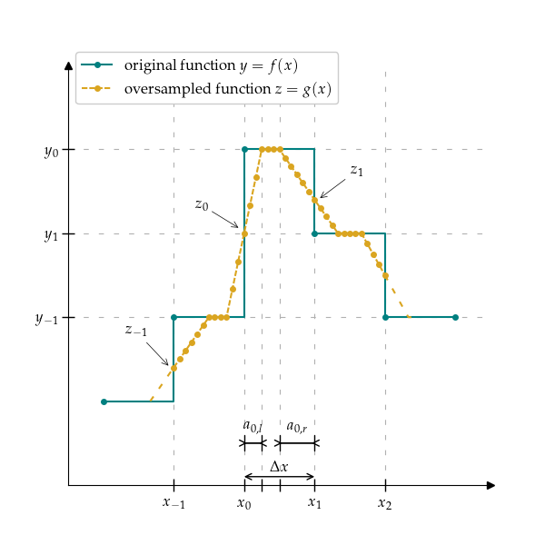
Transition linearly between intervals in transition window (part of the interval). Transition window is defined in number of samples a and divided according to the adaptive_factor. adaptive_factor is inversely proportionally to the change of function value on both edges of the interval, i.e., if function value has higher change on the right side of the interval, than on the left side, the right side transition window is smaller than the left one.

The impact of the adaptive_factor can be decreased by adjusting adaptive_smooth.

If a is not specified, it is obtained based on the transition samples factor alpha multiplied by the number of inserted samples for each interval n. a cannot be lower, than 2 samples. If it is, it’s value is changed to correct that.

Parameters:

x (1-D array-like) – Independent variable in strictly increasing order.
y (1-D array-like) – Dependent variable.
n (int) – Number of points oversampled and recreated in the function.
alpha (float, default: 1.0) – Transition window samples factor for moving between intervals.
a (int, optional) – Transition window samples for moving between intervals. If not specified, it is equal to alpha * n. Cannot be lower than 2.
adaptive_smooth (float, default: 1.0) – Decreasing impact of adaptive_factor by raising it to the power 1/adaptive_smooth.

Notes

Let us consider k-th interval and \(x_{k,i}\), \(y{k,i}\) refer to i-th sample of k-th interval for x and y, respectively. When omitting value, e.g., \(x_{k}\), it refers to the x_{k,0}.

Oversampling creates function \(z = g(x)\) from \(y=f(x)\).

Let assume, that:

the function is going to be oversampled with n samples in each interval.
\(\alpha\) is a given transition window factor parameter.
\(s\) is a given adaptive_smooth parameter
\(z_{k}\) is transition value between interval k and k - 1.
\(z_{k+1}\) is transition value between interval k and k + 1.
\(y_{k}\) is original function value in interval k.

Transition ranges depend on the change in function value between intervals.

1. When function changes between intervals, i.e., \(y_{k-1} \neq y_k \neq y_{k+1}\), an adaptive_factor \(\gamma_k\) and left and right transition windows \(a_k,l\) and \(a_k,r\) are calculated, as:

\[\begin{split}\gamma_k = \frac{|y_{1} - y_{0}|}{|y_{0} - y_{-1}|} ^ \frac{1/s} \\ \frac{a_{k,l}}{a_{k,r}} = \gamma_k \\ a_{k,l} = \min(\max(\frac{\gamma_k \cdot a}{1 + \gamma_k}, 1), a) \\ a_{k,r} = \min(\max(\frac{a}{1 + \gamma_k}, 1), a)\end{split}\]

The transition values are kept between 1 and n, thus:

\[\begin{split}a_{k,l} = \min(\max(a_{k,l}, 1) n) \\ a_{k,r} = \min(\max(a_{k,r}, 1) n) \\\end{split}\]

2. If function value is left and right side constant, i.e., \(y_{k-1} = y_k = y_{k+1}\), transition windows are calculated as:

\[a_{k, l} = a_{k, r} = 0\]

3. If function value is changing only on right side of the interval, i.e., \(y_{k-1} \neq y_k = y_{k+1}\),

\[a_{k, l} = 0 a_{k, r} = \frac{a}{2}\]

4. If function value is changing only on left side of the interval, i.e., \(y_{k-1} = y_k \neq y_{k+1}\),

\[a_{k, l} = \frac{a}{2} a_{k, r} = 0\]

Transition points and remaining points inside the interval are calculated same as in LinearFixedOversample().

\[\begin{split}\begin{cases} z_{k, i} = \mbox{lin_fit}(x_{k, i}, (x_{k, 0}, z_{k, 0}), (x_{k, a_{k, l}}, y_{k, 0})) & i \in \{0, a_l - 1\} \\ z_{k,i} = y_{k,i} & i \in \{a_{k,l}, n - a_r\} \\ z_{k, i} = \mbox{lin_fit}(x_{k, i}, (x_{k, n - a_{k, r}}, y_{k, 0}), (x_{k, n}, z_{k+1,0})) & i \in \{n - a_{k,r} + 1, n\} \end{cases}\end{split}\]

See also

LinearFixedOversample()

static get_adaptive_transition_points(x, y, a, adaptive_smooth)

Calculate transition points

Parameters:

x (IntervalArray) – independent variable
y (IntervalArray) – dependent variable
a (int) – transition window in samples
adaptive_smooth (float) – smoothing of adaptive_factor

Returns:

list of floats – Left transition window for each interval.
list of floats – Right transition window for each interval.
list of floats – Adaptive factor for each interval.

rfa()

Recreate function from average on x and y variables.

Returns:

xs (ndarray) – Oversampled independent variable x.
ys (ndarray) – Oversampled dependent variable y.

class ExpFixedRFA(x, y, n, alpha=1.0, beta=0.5, a=None, exp=2.0)

Bases: AbstractRFA

Moves between points in fixed transition intervals by combining linear and exponential function.

Transition combining linear and exponential function between intervals in transition window (part of the interval). Transition window is defined in number of samples a and divided proportionally to the left and right side of the interval. If a is not specified, it is obtained based on the transition samples factor alpha multiplied by the number of inserted samples for each interval n. a cannot be lower, than 2 samples. If it is, it’s value is changed to correct that.

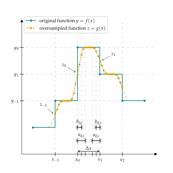
Left and right transition window is further divided into linear only part and combination of linear and exponential one. Division is done according to parameter beta and linear transition window is calculated as b = beta * a_l.

Parameters:

x (1-D array-like) – Independent variable in strictly increasing order.
y (1-D array-like) – Dependent variable.
n (int) – Number of points oversampled and recreated in the function.
alpha (float, default: 1.0) – Transition window samples factor for moving between intervals.
beta (float, default: 0.5) – Linear transition window samples factor.
a (int, optional) – Transition window samples for moving between intervals. If not specified, it is equal to alpha * n. Cannot be lower than 2.
exp (float, default: 2.0) – Exponent in exponential transition function.

Notes

Let us consider k-th interval and \(x_{k,i}\), \(y{k,i}\) refer to i-th sample of k-th interval for x and y, respectively. When omitting value, e.g., \(x_{k}\), it refers to the x_{k,0}.

Oversampling creates function \(z = g(x)\) from \(y=f(x)\).

Let assume, that: * the function is going to be oversampled with n samples in each interval. * \(\alpha\) is a given transition window factor parameter. * \(\beta\) is a given linear part of transition window factor parameter. * \(z_{k}\) is transition value between interval k and k - 1. * \(z_{k+1}\) is transition value between interval k and k + 1. * \(y_{k}\) is original function value in interval k.

Left \(a_l\) and right \(a_r\) transition number of samples is calculated as:

\[\begin{split}a = \alpha \cdot n \\ a_l = a_r = a / 2\end{split}\]

Let \(b\) denote Linear part of transition window, and it is calculated as:

\[b = \beta \cdot a_l\]

Transition points are calculated the same as in LinearFixedOversample().

Based on found transition values, remaining points in function \(z = g(x)\) are calculated as a linear combination of transition point and previous value using linear and exponential functions.

Two additional transition points are calculated, corresponding to \(x_{k, b}\) and \(x_{k, n - b}\) denoted as z_{k, b} and z_{k, n-b}. They are calculated as linear combination between \(z_{k, 0}\) and \(y_{k, 0}\), and \(z_{k+1, 0}\) and \(y_{k, 0}\), respectively.

\[\begin{split}\begin{cases} z_{k, i} = \mbox{lin_fit}(x_{k, i}, (x_{k, 0}, z_{k, 0}), (x_{k, b}, z_{k, b})) & i \in \{0, b - 1\} \\ z_{k, i} = \mbox{lin_exp_xy_fit}(x_{k, i}, (x_{k, b}, z_{k, b}), (x_{k, a_l}, y_{k, 0})) & i \in \{b, a_l - 1\} \\ z_{k,i} = y_{k,i} & i \in \{a_l, n - a_r\} \\ z_{k, i} = \mbox{exp_lin_fit}(x_{k, i}, (x_{k, n - a_r}, y_{k, 0}), (x_{k, n -b}, z_{k+1,n-b})) & i \in \{n - a_r + 1, n - b\} \\ z_{k, i} = \mbox{lin_fit}(x_{k, i}, (x_{k, n - b}, y_{k, n - b}), (x_{k, n}, z_{k+1,0})) & i \in \{n - b + 1, n\} \end{cases}\end{split}\]

where linfit linearly fits value based on two other points; lin_exp_xy_fit gradually fits combination of linear function and exponential function scaled from (0, 1) range and mirrored over y=x line; exp_lin_fit gradually fits combination of exponential function scaled from (0, 1) range and linear function.

See also

LinearFixedOversample(), lin_fit(), lin_exp_xy_fit(), exp_lin_fit()

rfa()

Recreate function from average on x and y variables.

Returns:

xs (ndarray) – Oversampled independent variable x.
ys (ndarray) – Oversampled dependent variable y.

class ExpAdaptiveRFA(x, y, n, alpha=1.0, beta=0.5, a=None, adaptive_smooth=1.0, exp=2.0)

Bases: AbstractRFA

Moves between points in adaptive transition intervals by combining linear and exponential function.

Transition combining linear and exponential function between intervals in transition window (part of the interval). Transition window is defined in number of samples a and divided according to the adaptive_factor. adaptive_factor is inversely proportionally to the change of function value on both edges of the interval, i.e., if function value has higher change on the right side of the interval, than on the left side, the right side transition window is smaller than the left one.

The impact of the adaptive_factor can be decreased by adjusting adaptive_smooth.

If a is not specified, it is obtained based on the transition samples factor alpha multiplied by the number of inserted samples for each interval n. a cannot be lower, than 2 samples. If it is, it’s value is changed to correct that.

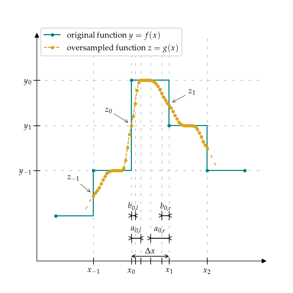
Left and right transition window is further divided into linear only part and combination of linear and exponential one. Division is done according to parameter beta and linear transition window is calculated as b = beta * a_l.

Parameters:

x (1-D array-like) – Independent variable in strictly increasing order.
y (1-D array-like) – Dependent variable.
n (int) – Number of points oversampled and recreated in the function.
alpha (float, default: 1.0) – Transition window samples factor for moving between intervals.
beta (float, default: 0.5) – Linear transition window samples factor.
a (int, optional) – Transition window samples for moving between intervals. If not specified, it is equal to alpha * n. Cannot be lower than 2.
adaptive_smooth (float, default: 1.0) – Decreasing impact of adaptive_factor by raising it to the power 1/adaptive_smooth.
exp (float, default: 2.0) – Exponent in exponential transition function.

Notes

This class combines functionality of LinearAdaptiveOversample() to calculate adaptive transition window, and ExpFixedOversample() to combine both linear and exponential function to change between intervals.

In particular, for each interval corresponding number of transition samples is calculated, respectively, and they are denoted as: \(a_{k, l}\), \(a_{k, r}\), \(b_{k, l}\), and \(b_{k, r}\).

Based on found transition values, remaining points in function \(z = g(x)\) are calculated as a linear combination of transition point and previous value using linear and exponential functions.

Two additional transition points are calculated, corresponding to \(x_{k, b}\) and \(x_{k, n - b}\) denoted as z_{k, b} and z_{k, n-b}. They are calculated as linear combination between \(z_{k, 0}\) and \(y_{k, 0}\), and \(z_{k+1, 0}\) and \(y_{k, 0}\), respectively.

Then the points in interval are calculated as:

\[\begin{split}\begin{cases} z_{k, i} = \mbox{lin_fit}(x_{k, i}, (x_{k, 0}, z_{k, 0}), (x_{k, b_{k, l}}, z_{k, b_{k, l}})) & i \in \{0, b_{k, l} - 1\} \\ z_{k, i} = \mbox{lin_exp_xy_fit}(x_{k, i}, (x_{k, b_{k, l}}, z_{k, b_{k, l}}), (x_{k, a_{k, l}}, y_{k, 0})) & i \in \{b_{k, l}, a_{k, l} - 1\} \\ z_{k,i} = y_{k,i} & i \in \{a_{k, l}, n - a_{k, r}\} \\ z_{k, i} = \mbox{exp_lin_fit}(x_{k, i}, (x_{k, n - a_{k, r}}, y_{k, 0}), (x_{k, n - b_{k, r}}, z_{k+1,n-b_{k,r}})) & i \in \{n - a_{k, r} + 1, n - b_{k,r}\} \\ z_{k, i} = \mbox{lin_fit}(x_{k, i}, (x_{k, n - b_{k,r}}, y_{k, n - b_{k, r}}), (x_{k, n}, z_{k+1,0})) & i \in \{n - b_{k,r} + 1, n\} \end{cases}\end{split}\]

where linfit linearly fits value based on two other points; lin_exp_xy_fit gradually fits combination of linear function and exponential function scaled from (0, 1) range and mirrored over y=x line; exp_lin_fit gradually fits combination of exponential function scaled from (0, 1) range and linear function.

See also

LinearFixedOversample(), lin_fit(), lin_exp_xy_fit(), exp_lin_fit()

rfa()

Recreate function from average on x and y variables.

Returns:

xs (ndarray) – Oversampled independent variable x.
ys (ndarray) – Oversampled dependent variable y.